Tutorial#

Every code based on Hiperwalk follows up to five distinct steps.

Import the Hiperwalk package.
Define a graph.
Construct the quantum walk using the previously defined graph.
Run the simulation of the quantum walk.
Display the results.

An easy-to-understand example is the coined walk on the line. Don’t worry about the specifics for the time being; we are merely illustrating the steps.

Import the Hiperwalk package#

>>> import hiperwalk as hpw

Define a graph#

In this step, we generate a line comprising 11 vertices. The output is an object from the hiperwalk.Line class.

>>> N = 11
>>> line = hpw.Line(N)
>>> line 
<hiperwalk.graph.line.Line object at 0x7ff59f1900d0>

Construct the quantum walk using the previously defined graph#

We now create a coined quantum walk on the line with 11 vertices. We achieve this by passing the previously created graph as an argument to the quantum walk constructor. The outcome is an object from the hiperwalk.Coined class.

>>> qw = hpw.Coined(line)
>>> qw 
<hiperwalk.quantum_walk.coined_walk.Coined object at 0x7f2691de9840>

Simulate the quantum walk#

Before running the simulation, we need to specify the initial state. One way to accomplish this is by using the hiperwalk.Coined.ket() method, which generates a state of the computational basis.

>>> vertex = N // 2
>>> state = qw.ket((vertex, vertex + 1))
>>> state
array([0., 0., 0., 0., 0., 0., 0., 0., 0., 1., 0., 0., 0., 0., 0., 0., 0.,
       0., 0., 0.])

This state corresponds to the walker on vertex 5 with the coin pointing to vertex 6 (keep in mind that the vertex numbers range from 0 to 10).

To run the simulation, we must specify the initial state and the number of steps (i.e., the number of applications of the evolution operator). When specifying only the final time, the output will be the final state. If everything was installed correctly, the hiperwalk.Coined.simulate() method will automatically use high-performance computing to perform the matrix-vector multiplications.

>>> final_state = qw.simulate(time=N//2,
...                           state=state)

Display the results#

Presenting the results can be as straightforward as printing them.

>>> final_state
array([[ 0.1767767 ,  0.        ,  0.        , -0.1767767 ,  0.35355339,
         0.        ,  0.        ,  0.        , -0.35355339,  0.        ,
         0.        ,  0.        ,  0.35355339,  0.        ,  0.        ,
         0.70710678,  0.1767767 ,  0.        ,  0.        ,  0.1767767 ]])

Or, the output could be more sophisticated. Often, we are interested in the probability of the walker being found at each vertex. This can be accomplished via the hiperwalk.Coined.probability_distribution() method by passing the final state as an argument.

>>> probability = qw.probability_distribution(final_state)
>>> probability
array([[0.03125, 0.     , 0.15625, 0.     , 0.125  , 0.     , 0.125  ,
        0.     , 0.53125, 0.     , 0.03125]])

It’s also feasible to plot the probability distribution using a simple command.

>>> hpw.plot_probability_distribution(probability) 

This command generates the following plot:

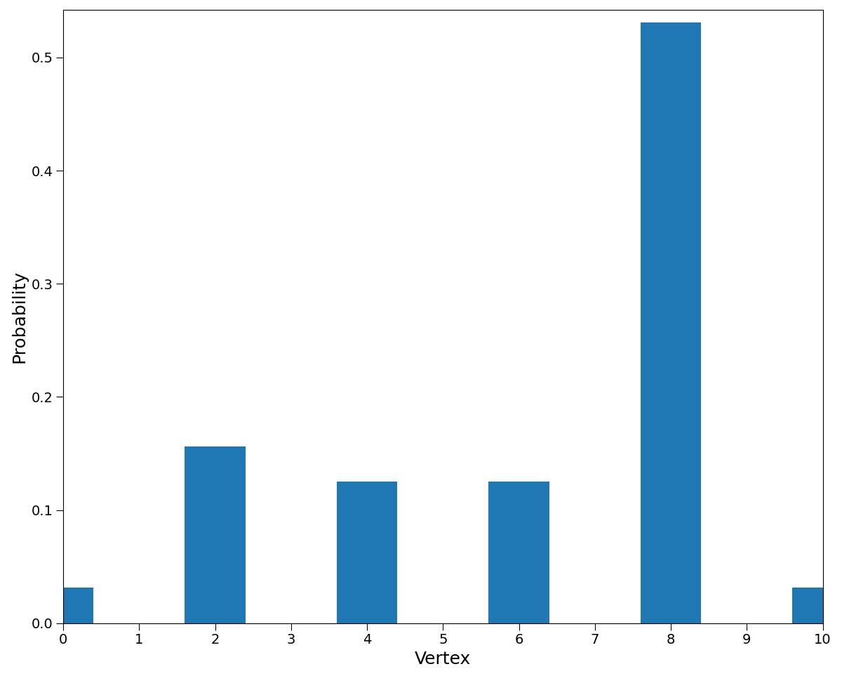
Plot of the probability distribution. — Probability distribution of a quantum walk on a line.#

Next Steps#

The remainder of the tutorial is split into the following sections.